Numerical methods
The library relies on the data model and the workflow proposed in Mordicus, see the Mordicus methodology documentation for details.
The main feature of genericROM is the nonlinear projection-based model-order reduction, using snapshot Proper Orthogonal Decomposition (snapshot-POD) for the data compression, and Empirical Cubature Method (ECM) for the operator compression steps. We briefly illustrate the main concepts here for nonlinear structural mechanics. More details being available in the Section Publications (article 1 for nonlinear structural mechanics; article 2 for nonlinear transient thermal problems).
High-Fidelity Model (HFM)
Consider a structure denoted \(\Omega\), whose boundary \(\partial\Omega\) is partitioned as \(\partial\Omega=\partial\Omega_D\cup\partial\Omega_N\) such that \(\partial\Omega_D^{\mathrm{o}}\cap\partial\Omega_N^{\mathrm{o}}=\emptyset\), see Fig. 1.
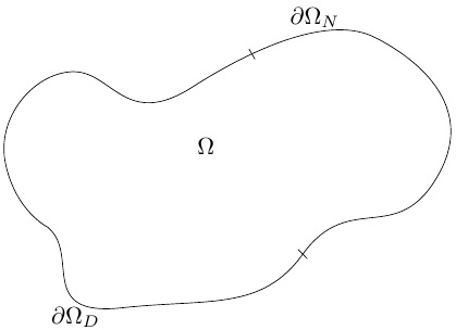
Fig. 1 Schematic representation of the structure of interest.
The structure is subjected to a quasi-static time-dependent loading, composed of an homogeneous Dirichlet boundary conditions on \(\partial\Omega_D\) and Neumann boundary conditions on \(\partial\Omega_N\) in the form of a prescribed traction \(T_N\), as well as a volumic force \(f\). The setting depends on some variability \(\mu\), which can be a parameter vector, or represent some nonparametrized variability. The evolution of the displacement \(u_\mu(x,t)\) over \((x,t)\in\Omega\times[0,T]\) is governed by equations:
where \(\epsilon\) is the linear strain tensor, \(\sigma_\mu\) is the Cauchy stress tensor, \(y_\mu\) denotes the internal variables of the constitutive law and \(n_{\partial\Omega}\) is the outward normal vector on \(\partial\Omega\). We precise that the evolution of the internal variables \(y_\mu\) is updated while solving the constitutive law.
Define \(H^1_0(\Omega)=\{v\in L^2(\Omega)|~\frac{\partial v}{\partial x_i}\in L^2(\Omega),~1\leq i\leq 3{\rm~and~}v|_{\partial\Omega_D}=0\}\). Denote \(\{\varphi_i\}_{1\leq i\leq N}\in\mathbb{R}^{N\times N}\), a finite element basis whose span, denoted \(\mathcal{V}\), constitutes an approximation of \(H^1_0(\Omega)^3\); \(N\) is the number of finite element basis functions, hence the number of degrees of freedom of the discretized prediction. A discretized weak formulation reads: find \(u_\mu\in \mathcal{V}\) such that for all \(v\in \mathcal{V}\),
that we denote for concision \(\mathcal{F}_\mu\left(u_\mu\right)=0\). A Newton algorithm can be used to solve this nonlinear global equilibrium problem at each time step:
where
and
In the two relations above, \(\mathcal{K}\left(\epsilon(u_\mu^k),y_\mu\right)\) is the local tangent operator, \(u_\mu^k\in\mathcal{V}\) is the k-th iteration of the discretized displacement field at the current time-step, and \(\boldsymbol {u}_\mu^k=\left(u_{\mu,i}^k\right)_{1\leq i\leq N}\in\mathbb{R}^N\) is such that \(\displaystyle u_\mu^k=\sum_{i=1}^Nu_{\mu,i}^k\varphi_i\). In particular, \(f_\mu\), \(T_{\mu,N}\), \(u_\mu^k\) and \(y_\mu\) are known and enforce the time-dependence of the solution. Depending on the constitutive law, the computation of the functions \(\displaystyle\left(u_\mu^k,y\right)\mapsto \sigma\left(\epsilon(u_\mu^k),y_\mu\right)\) and \(\displaystyle\left(u_\mu^k,y\right)\mapsto \mathcal{K}\left(\epsilon(u_\mu^k),y_\mu\right)\) can involve complex differential-algebraic system of equations.
Projection-based Reduced-Order Modeling (ROM)
The object of this section is to provide synthetic elements on the numerical methods, and some implementation choices made in the library genericROM.
As explained in Mordicus methodology documentation, usual ROM workflows contain an offline (learning) phase and an online (exploitation) phase.
We start by explaining the online phase and presenting the ROM. Since we want to construct and solve it in the most efficient way, the offline phase is dedicated to precompute as many steps as possible, under the considered variability.
Online phase
The reduced-order model is obtained by assembling the physical problem in the same fashion as the HFM in Section High-Fidelity Model (HFM), with the difference that the finite element basis \((\varphi_i)_{1\leq i\leq N}\in\mathbb{R}^{N\times N}\), is replaced by a reduced-order basis (ROB) \((\psi_i)_{1\leq i\leq n}\in\mathbb{R}^{n\times N}\), with \(n\ll N\). Hence, the reduced Newton algorithm is constructed as
where
and
In the two relations above, \(\hat{u}_\mu^k\in\hat{\mathcal{V}}:={\rm Span}\left(\psi_i\right)_{1\leq i\leq n}\) is the \(k\)-th iteration of the reduced displacement field for the current time-step and \(\hat{\boldsymbol{u}}_\mu^k=\left(\hat{u}^k_{\mu, i}\right)_{1\leq i\leq n}\in\mathbb{R}^n\) is such \(\displaystyle\hat{u}_\mu^k=\sum_{i=1}^n\hat{u}^k_{\mu, i}\psi_i\).
The online stage is said efficient if the reduced problem can be constructed and solved in computational complexity independent of \(N\). When the variability \(\mu\) is parametrized, efficiency is possible by precomputing various terms. With nonparametrized variability, depending on its nature, some assembling task with a linear complexity in \(N\) may be required at the beginning of the online stage (for instance for a boundary condition). All these scenarios are handled by genericROM.
The offline phase contains three steps, for which we present below the methodological choices made in genericROM, as well as intuition and implementation details.
Offline phase
Data generation
This step corresponds to the generation of the snapshots by solving the high-fidelity model. In genericROM, projection-based ROMs can be constructed even when the snapshots are generated by commercial software, as long as a reader for the computed solution is available (or can be developed).
Data compression
This step corresponds to the generation of the ROB \((\psi_i)_{1\leq i\leq n}\). The simplest method available in genericROM is the snapshot-POD:
Choose a tolerance \(\epsilon_{\rm POD}\).
Compute the correlation matrix \(C_{i,j}=\int_{\Omega}u_i\cdot u_j\), \(1\leq i,j\leq N_s\), where \(N_s\) is the total number of HFM snapshots.
Compute the \(\epsilon_{\rm POD}\)-truncated eigendecomposition of \(C\): \(\xi_i\in\mathbb{R}^{N_c}\) and \(\lambda_i>0\), where \(1\leq i\leq n\), are the \(n\) first eigenvector and eigenvalues.
Compute the reduced order basis \(\displaystyle\psi_i(x)=\frac{1}{\sqrt{\lambda_i}}\sum_{j=1}^{N_s}u_j(x){\xi_i}_j\), \(1\leq i\leq n\).
The snapshot-POD is also available in parallel with distributed memory, by partitioning the domain \(\Omega\) in subdomains.
Operator compression
This step corresponds to the additional treatment needed to guarantee the efficiency of the online stage, by pre-processing of the computationally demanding integration over \(\Omega\) and \(\partial\Omega_N\). Notice that for computing the reduced Newton algorithm in Section Online phase, without additional approximation, the numerical integration step will in practice strongly limit the efficiency of the ROM (no interesting speedup with respect to the computation of the high-fidelity model will be obtained in practice). In genericROM, an implementation of the Empirical Cubature Method (ECM) is available to tackle this problem. A concise description is given below, more details are available in Section Publications, article 1.
In the finite element method, the integrals in the HFM are computed using high-fidelity quadrature formulas, which, when applied to the reduced internal forces vector, read
where \(E\) denotes the set of elements of the mesh, \(n_e\) the number of integration points for the element \(e\), \(\omega_k\) and \(x_k\) are the integration weights and points of the considered element. We define \(N_G\) the total number of integration points.
The ECM consists in replacing the high-fidelity quadratures by a reduced quadrature with positive weights, which, when applied to the reduced internal forces vector, read
where \(\hat{\omega}_{k'}>0\) and \(\hat{x}_{k'}\) are respectively the reduced integration weights and points, and \(n_g\ll N_G\) is the length of the reduced quadrature.
Computation of the reduced quadrature:
Denote \(f_q:=\sigma\left(\epsilon(u_{(q//n)+1}),y\right):\epsilon\left(\psi_{(q\%n)+1}\right)\), \(1\leq q\leq nN_c\). where \(//\) and \(\%\) denote respectively the quotient and the remainder of the Euclidean division. Denote also \(\mathcal{Z}^{n_G}\) a subset of \([1;N_G]\) of size \(n_G\) and \(J_{\mathcal{Z}^{n_G}}\in\mathbb{R}^{nN_c\times n_G}\) and \(\boldsymbol{b}\in\mathbb{N}^{nN_c}\) such that for all \(1\leq q\leq nN_c\) and all \(1\leq q'\leq n_G\),
where \(\mathcal{Z}^{n_G}_{q'}\) denotes the \(q'\)-th element of \(\mathcal{Z}^{n_G}\). Recall that \(n\) is the number of snapshot POD modes. Let \(\hat{\boldsymbol{\omega}}\in{\mathbb{R}^{+}}^n_G\), \(\displaystyle\left(J_{\mathcal{Z}^{n_G}}\hat{\boldsymbol{\omega}}\right)_q=\sum_{q'=1}^{n_G}\hat{\omega}_{q'}\sigma\left(\epsilon(u_{{(q//n)+1}}),y\right)(x_{\mathcal{Z}^{n_G}_{q'}}):\epsilon\left(\psi_{(q\%n)+1}\right)(x_{\mathcal{Z}_{q'}})\), \(1\leq q\leq nN_c\) is a candidate approximation for \(\displaystyle \int_{\Omega}\sigma\left(\epsilon(u_{{(q//n)+1}}),y\right):\epsilon\left(\psi_{(q\%n)+1}\right) = b_q`~, :math:`1\leq q\leq nN_c\). The problem of finding the best reduced quadrature formula of length \(n_G\) for the reduced internal forces vector can be written:
where \(\left\|\cdot\right\|\) stands for the Euclidean norm. Taking the length of the reduced quadrature formula in the objective function of the optimization leads to a NP-hard problem, which in approximately solved in genericROM using an Nonnegative Orthogonal Matching Pursuit algorithm.
Implementation details
Noninstrusivity
GenericROM enables the handling of projection-based ROM workflow in a nonintrusive manner: the user do not need to modify assembling routine of the reference code used to solve the HFM. For instance, ROM can be constructed using data generated by commercial code like Ansys and Abaqus can be used (see Publications, article 2, for the construction of a ROM for nonlinear transient thermal problem using data generated by Abaqus). To do so, the assembling routine of operators and right-hand side are handling directly in genericROM, using the finite element engine of Muscat developped at Safran.
Precomputations for efficiency
In ROM workflows, the common measure of efficiency is the speedup, defined as the ratio between the computation duration of the HFM and the one of the ROM. For a given accuracy, the higher the speedup, the better. Various elements can be taken into account, including code optimization of the online stage.
The methods enabling algorithmic complexity gains have been presented in Section Offline phase. In this section, we give additional implementation elements and illustrations to give some intuition on the mechanisms at play.
Depending on the considered equations and nature of variability, the goal is to precompute as many quantities as possible in the offline stage, to leave as few operations as possible to the online stage.
In the HFM, the assembling of the global tangent operator at each Newton iteration, using the high-fidelity quadrature, reads:
In the proposed ROM, the assembling of the reduced global tangent operator at each Newton iteration, using the reduced quadrature, reads:
The corresponding linear systems are illustrated on Fig. 2 and Fig. 3. In particular, \(n\) should be much smaller than \(N\) to obtain a significant speedup despite the fact that the linear system is sparse in the HFM and dense in the ROM.
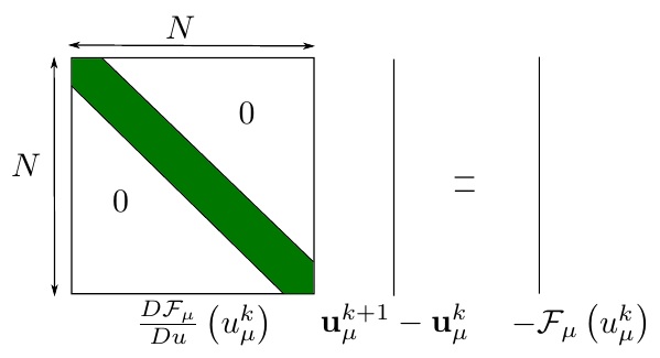
Fig. 2 HFM: a large sparse linear system is assembled and solved at each step of the Newton algorithm.

Fig. 3 ROM: a small dense linear system is assembled and solved at each step of the reduced Newton algorithm.
Based on Fig. 2 and Fig. 3, the speedup is clear for the resolution part of the linear system. We still need to illustrate how precomputations in the offline phase allow an efficient assembling of the reduced problem. Denote \(d\) the number of unknowns of second-order tensor dual quantities. In 3D, \(d=6\), for instance for the strain tensor, the unknowns are \(\epsilon_{11}, \epsilon_{22}, \epsilon_{33}, \epsilon_{12}, \epsilon_{23}, \epsilon_{31}\). The reduced global tangent operator at each Newton iteration, using the reduced quadrature, can be written
In genericROM, the code for computing this quantity in the online stage is
reducedTangentMatrix = np.einsum('g,lgj,glm,mgi->ij', reducedIntegrationWeights, reducedEpsilonAtReducedIntegPoints,
                                 localTgtMat, reducedEpsilonAtReducedIntegPoints, optimize = True)
where
reducedIntegrationWeights[g]= \(\omega_g\),reducedEpsilonAtReducedIntegPoints[lgj]= \(\epsilon_l\left(\psi_j\right)\left(\hat{x}_g\right)\),localTgtMat[glm]= \(\mathcal{K}_{l,m}\left(\epsilon(\hat{u}_\mu^k),y_\mu\right)\left(\hat{x}_g\right)\).
The object reducedEpsilonAtReducedIntegPoints is a third-order tensor containing the components of the strain tensor applied to the ROB and
evaluated at the reduced integration points. This quantity is precomputed in the offline stage.
The object localTgtMat is a third-order tensor containing the components of the local tangent matrix evaluated at the reduced integration points:
this quantity is computed online by the constitutive law solver.
Publications
The numerical illustrations in the following articles have been computed using genericROM (or a previous version of the library). In particular, the methology for the mechanical and thermal reduced order modeling are detailed respectively in the first two articles:
Number |
Informations |
Illustration |
|---|---|---|
1 |
|

|
2 |
|
|
3 |
|

|
4 |
|

|
5 |
|
|
6 |
|
|
7 |
|

|
8 |
|

|