ThermalSequential

The data needed to execute the tutorials below can be loaded here: exampleThermalSequential.zip

This use case aims to validate the methodology POD + ECM for nonlinear transient thermal computations, see Section Publications, article 2.

No optional prerequisite: notice that even if the HFM snapshots are computed here using Z-set, the ROM do not require any Z-set license to be run.

Description of the physics problem

Geometry, loading and boundary condtions

Consider a 1m-wide 2D square, illustrated in Fig. 16. Let \(t_f\) denote the last time step, the square is subjected to

• a radiation boundary condition at \(\Gamma\): \(q_{\rm rad}(x,t)\cdot n(x)=\sigma\epsilon\left(T^4(x,t)-T^4_{2,e}(t)\right)\), for \((x,t)\in\Gamma\times[0,t_f]\),

• a convective heat flux boundary condition at \(\Gamma\): \(q_{\rm conv}(x,t)\cdot n(x)=h\left(T(x,t)-T_{1,e}(t)\right)\), for \((x,t)\in\Gamma\times[0,t_f]\),

where \(h\) denotes the convection coefficient (in J.s^-1.m^-2.K^-1), \(\sigma\) the Stefan–Boltzmann constant (in J.s^-1.m^-2.K^-4), \(\epsilon\) is the emissivity coefficient (dimensionless), \(T_{1,e}\) and \(T_{2,e}\) are external temperature values.

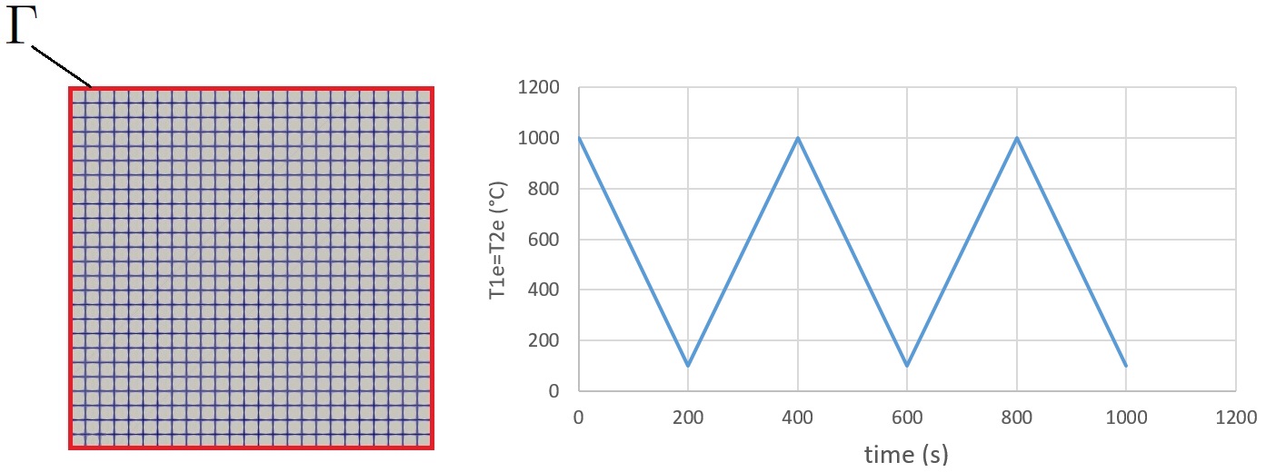
Fig. 16 (left) 2D-mesh of the test case, (right) profile of the \(T_{1,e}=T_{2,e}\) parameter of the convective heat flux boundary condition with respect to time.

Modeling hypothesis

Transient heat equation.

Material behavior

The material is modeled by piecewise linear profiles of the heat conductivity and capacity with respect to the solution temperature. The (purposely irregular) profiles taken for the example are illustrated on Fig. 17.

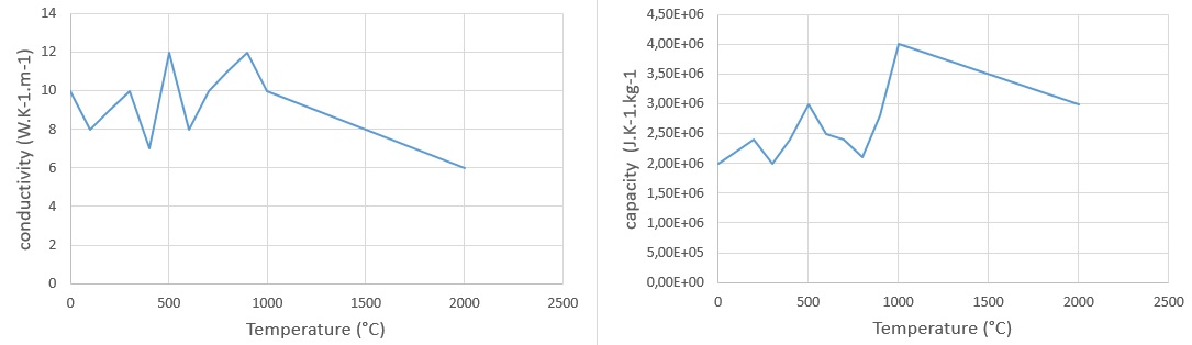
Fig. 17 Constitutive law model: (left) heat conductivity (W.K^-1.m^-1) and (right) heat capacity (J.K^-1.kg^-1) with respect to the temperature (°C).

Reduction strategy

Inputs and outputs

This is a simple “reproducting use case”, where a reduced-order model is constructed to reproduce a high-fidelity solution and check its quality. This use case contains the modeling complexity of the high-pressure turbine blade cyclic extrapolation, except for the parallel computation in distributed memory and the fact that the turbine features two material (elastic and elastoviscoplastic).

The number of simulation cycles can be seen as the input, while the outputs are the displacement field U and the accumulated plasticity field \(p\) (named evrcum).

Data compression

The reduced-order basis is generated by the snapshot-POD method CompressData from the DataCompressors.FusedSnapshotPOD module.

Operator compression

The operator compression step is computed using the ECM (Empirical Cubature Method) CompressOperator from the OperatorCompressors.Thermal_transient module. More precisely, the ECM is used three time, to approximate the nonlinear terms obtained by the nonlinearity of the heat conductivity and capacity, and the radiation boundary condition term.

Algorithm

Results formats and simulation codes

Snapshots are generated by Z-set and read from the Z-set format.

Quality approximation verification

The quality of the data compression is evaluated by computed the relative projection error of the high-fidelity solutions on the reduced-order basis:

\[\dfrac{\left\|T - \sum_{i=1}^N \left( T, \Psi_i^T\right) \Psi_i^T\right\|}{\left\|T\right\|} \le 1 \times 10^{-5},\]

where \(\Psi_i^T\) denote the POD modes (or vectors of the reduced-order basis). The same quantity is considered from \(p\).

The quality of the complete procedure is evaluated by compute the relative \(\mathcal{l}_2\)-norm error between the high-fidelity solutions and the reduced ones:

\[\dfrac{\left\|T - \sum_{i=1}^N \gamma_i^T \Psi_i^T\right\|}{\left\|T\right\|} \le 2 \times 10^{-3},\]

with \(\gamma_i^T\) the coefficients of the reduced solution (or reducedCoordinates) computed by the reduced-order model.

Code - offline stage

List of imports required for the offline stage of this example:

from genericROM.IO import ZsetInputReader as ZIR
from genericROM.IO import ZsetMeshReader as ZMR
from genericROM.IO import ZsetSolutionReader as ZSR
from Mordicus.Containers import ProblemData as PD
from Mordicus.Containers import CollectionProblemData as CPD
from Mordicus.Containers import Solution as S
from genericROM.FE import FETools as FT
from genericROM.DataCompressors import FusedSnapshotPOD as SP
from genericROM.OperatorCompressors import Thermal_transient as Th
from Mordicus.IO import StateIO as SIO
from Mordicus.Helpers import FolderHandler as FH
from genericROM import GetTestDataPath
import numpy as np
import os

Then, filename and dimensions related to the mesh and the solutions have to be declared, readers are initalized, and the mesh is read:

folder = GetTestDataPath()+"Zset"+os.sep+"ThermalSequential"+os.sep

meshFileName = folder + "square.geof"
inputFileName = folder + "square.inp"
solutionFileName = folder + "square.ut"

meshReader = ZMR.ZsetMeshReader(meshFileName)
inputReader = ZIR.ZsetInputReader(inputFileName)
solutionReader = ZSR.ZsetSolutionReader(solutionFileName)

mesh = meshReader.ReadMesh()
numberOfNodes = mesh.GetNumberOfNodes()
nbeOfComponentsPrimal = 1

Then, the part of the ECM algorithm depending only on the mesh is carried out:

operatorPreCompressionData = Th.PreCompressOperator(mesh, "ALLBOUNDARY")

Then, the objects Solution are declared and populated with data from the precomputed Z-set solutions:

outputTimeSequence = solutionReader.ReadTimeSequenceFromSolutionFile()
solutionT = S.Solution("T", nbeOfComponentsPrimal, numberOfNodes, primality = True)
for time in outputTimeSequence:
    T = solutionReader.ReadSnapshot("TP", time, nbeOfComponentsPrimal, primality=True)
    solutionT.AddSnapshot(T, time)

Then, the constitutive laws, required for ECM in thermal problems, are read:

constitutiveLawsList = inputReader.ConstructConstitutiveLawsList()

Then, the objects CollectionProblemData and ProblemData are declared, which will enable to agregate the Solution objects previously constructed in a standard fashion in Mordicus:

problemData = PD.ProblemData(folder)
problemData.AddSolution(solutionT)
problemData.AddConstitutiveLaw(constitutiveLawsList)

collectionProblemData = CPD.CollectionProblemData()
collectionProblemData.AddVariabilityAxis("config", str)
collectionProblemData.DefineQuantity("T", "temperature", "K")
collectionProblemData.AddProblemData(problemData, config="case-1")

Then, the \(L_2 (\Omega)\) correlation operator between snapshots is computed (identified by “T”):

snapshotCorrelationOperator = {"T": FT.ComputeL2ScalarProducMatrix(mesh, 1)}

Then, using the snapshots-POD method, we compute the reduced-order basis for the solutions T with the \(L_2 (\Omega)\) correlation operator, and compress the snapshots on this reduced-order basis:

SP.CompressData(collectionProblemData, "T", 1.e-6, snapshotCorrelationOperator["T"], compressSolutions = True)

Then, we verify the quality of the data compression on T as explained in :

reducedOrderBasisT = collectionProblemData.GetReducedOrderBasis("T")
CompressedSolutionT = solutionT.GetReducedCoordinates()

compressionErrors = []
for t in outputTimeSequence:
    reconstructedCompressedSolution = np.dot(CompressedSolutionT[t], reducedOrderBasisT)
    exactSolution = solutionT.GetSnapshot(t)
    norml2ExactSolution = np.linalg.norm(exactSolution)
    if norml2ExactSolution != 0:
        relError = np.linalg.norm(reconstructedCompressedSolution-exactSolution)/norml2ExactSolution
    else:
        relError = np.linalg.norm(reconstructedCompressedSolution-exactSolution)
    compressionErrors.append(relError)

Then, we carry out the ECM algorithm to determine the reduced quadrature schemes:

Th.CompressOperator(collectionProblemData, operatorPreCompressionData, mesh, 1.e-5)

Finally, at the end of the offline, the Modicus data model containing the results of this stage, is saved on disk in order to used them during the online stage.

SIO.SaveState("collectionProblemData", collectionProblemData)
SIO.SaveState("snapshotCorrelationOperator", snapshotCorrelationOperator)

Code - online stage

List of imports required for the offline stage of this example:

from genericROM.IO import ZsetInputReader as ZIR
from genericROM.IO import ZsetMeshReader as ZMR
from genericROM.IO import ZsetSolutionReader as ZSR
from genericROM.IO import ZsetSolutionWriter as ZSW
from Mordicus.Containers import ProblemData as PD
from Mordicus.Containers import Solution as S
from genericROM.IO import PXDMFWriter as PW
from genericROM.OperatorCompressors import Thermal_transient as Th
from Mordicus.IO import StateIO as SIO
from Mordicus.Helpers import FolderHandler as FH
from genericROM import GetTestDataPath
import numpy as np
import os

First, data saved on disk at the end of the offline stage is read:

collectionProblemData = SIO.LoadState("collectionProblemData")
operatorCompressionData = collectionProblemData.GetOperatorCompressionData("T")
snapshotCorrelationOperator = SIO.LoadState("snapshotCorrelationOperator")
reducedOrderBases = collectionProblemData.GetReducedOrderBases()

Then, filename and dimensions related to the mesh and the solutions have to be declared and readers are initalized, in the same fashion as the offline stage. We mention here that the physical setting for the online stage has been taken identical to the one used in the offline stage (the folder “ThermalSequential/”). In meaningful workflow, the physical setting for the online stage would be different.

folder = GetTestDataPath()+"Zset"+os.sep+"ThermalSequential"+os.sep
inputFileName = folder + "square.inp"
inputReader = ZIR.ZsetInputReader(inputFileName)
meshFileName = folder + "square.geof"

Then, the mesh is read (which is required when the variability is not parametrized):

mesh = ZMR.ReadMesh(meshFileName)

Then, an object ProblemData is defined, which will store the data computed during the online stage:

onlineProblemData = PD.ProblemData("Online")
onlineProblemData.SetDataFolder(os.path.relpath(folder, folderHandler.scriptFolder))

Then, the temporal sequence and the constitutive law are read from the Z-Set input file. These are “fixed data” for the online resolution:

timeSequence = inputReader.ReadInputTimeSequence()
constitutiveLawsList = inputReader.ConstructConstitutiveLawsList()
onlineProblemData.AddConstitutiveLaw(constitutiveLawsList)

Then, the loadings and initial condition are read from the Z-Set input file and are reduced by projecting them onto the reduced-order basis:

loadingList = inputReader.ConstructLoadingsList()
onlineProblemData.AddLoading(loadingList)
for loading in onlineProblemData.GetLoadingsForSolution("T"):
    loading.ReduceLoading(mesh, onlineProblemData, reducedOrderBases, operatorCompressionData)

initialCondition = inputReader.ConstructInitialCondition()
onlineProblemData.SetInitialCondition(initialCondition)
initialCondition.ReduceInitialSnapshot(reducedOrderBases, snapshotCorrelationOperator)

Then, the reduced solution is computed in a nonintrusive fashion using a reduced Newton iterative algorithm for solving the reduced nonlinear system of equations at each time-step:

onlineReducedCoordinates = Th.ComputeOnline(onlineProblemData, timeSequence, operatorCompressionData, 1.e-5)

Then, the reduced solution is written on disk, and the accuracy is checked in the same fashion as in the tutorial MecaSequential.

Results

A comparison between the reduced and reference high-fidelity solutions is illustrated in Fig. 18.

In Fig. 18, the quality of the reduced model is illustrated by comparing it to the high-fidelity reference. The comparison is done on the temperature field.

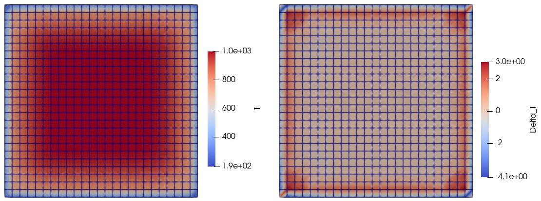
Fig. 18 Illustration of the ROM accuracy on the temperatre T (left) HFM, (right) pointwise difference between the ROM and the HFM.