MecaSequential

This use case aims to validate the methodology POD + ECM for quasistatic elastoviscoplastic computations with Z-set, with a reconstruction of the dual quantities using the gappy POD, see Section Publications, article 1.

Optional prerequisite: Zmat.

The data needed to execute the tutorials below can be loaded here: exampleMecaSequential.zip

Description of the physics problem

Geometry, loading and boundary condtions

Consider a 1m-wide cube, illustrated in Fig. 4. This cube is subjected to

• a variable thermal loading, in the form of time- and space-dependant scalar field obtained from a previous thermal computation, see Fig. 4 (right)

• a centrifugal effect generated by a rotation along the \(Z\)-axis

• a time- and space-dependant pressure filed applied on the \(X_1\) face

• fixed displacement imposed along the \(X\)-axis on the \(X_0\) face, along the \(Y\)-axis on the \(X_0Y_0\) edge and along the \(Z\)-axis on the \(X_0Y_1Z_1\) vertex

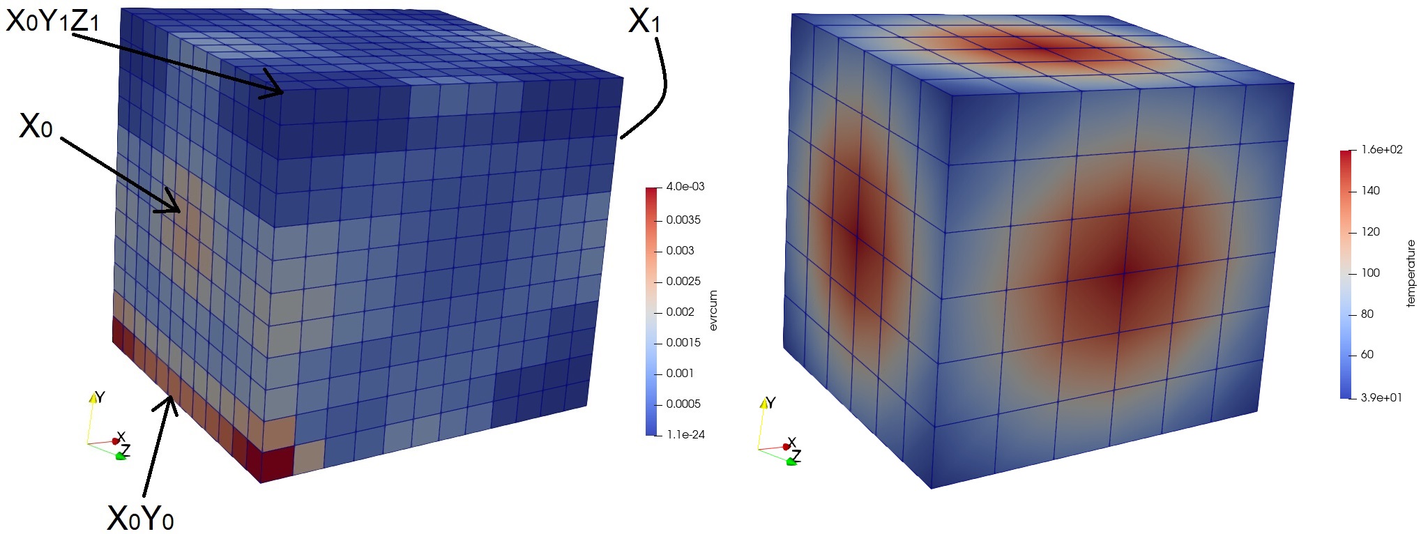
Fig. 4 (left) Dual mesh of the test case with the accumulated plasticity filed at the end of the simulation, (right) mesh and maximal temperature loading field.

Modeling hypothesis

Quasistatic equilibrium equations for the deformable solide in small perturbations.

Material behavior

The material is elastoviscoplastic with nonlinear hardening and a Norton flow. The constitutive law is specified by the .mat file.

Reduction strategy

Inputs and outputs

This is a simple “reproducting use case”, where a reduced-order model is constructed to reproduce a high-fidelity solution and check its quality. This use case contains the modeling complexity of the high-pressure turbine blade cyclic extrapolation, except for the parallel computation in distributed memory and the fact that the turbine features two material (elastic and elastoviscoplastic).

The number of simulation cycles can be seen as the input, while the outputs are the displacement field U and the accumulated plasticity field \(p\) (named evrcum).

Data compression

The reduced-order basis is generated by the snapshot-POD method CompressData from the DataCompressors.FusedSnapshotPOD module.

Operator compression

The operator compression step is computed using the ECM (Empirical Cubature Method) CompressOperator from the OperatorCompressors.Mechanical module.

Algorithm

Results formats and simulation codes

Snapshots are generated by Z-set and read from the Z-set format.

Quality approximation verification

The quality of the data compression is evaluated by computed the relative projection error of the high-fidelity solutions on the reduced-order basis:

\[\dfrac{\left\|u - \sum_{i=1}^N \left( u, \Psi_i^u\right) \Psi_i^u\right\|}{\left\|u\right\|} \le 1 \times 10^{-5},\]

where \(\Psi_i^u\) denote the POD modes (or vectors of the reduced-order basis). The same quantity is considered from \(p\).

The quality of the complete procedure is evaluated by compute the relative \(\mathcal{l}_2\)-norm error between the high-fidelity solutions and the reduced ones:

\[\dfrac{\left\|u - \sum_{i=1}^N \gamma_i^u \Psi_i^u\right\|}{\left\|u\right\|} \le 1 \times 10^{-5},\]

with \(\gamma_i^u\) the coefficients of the reduced solution (or reducedCoordinates) computed by the reduced-order model.

Code - offline stage

List of imports required for the offline stage of this example:

from genericROM.IO import ZsetMeshReader as ZMR
from genericROM.IO import ZsetSolutionReader as ZSR
from Mordicus.Containers import ProblemData as PD
from Mordicus.Containers import CollectionProblemData as CPD
from Mordicus.Containers import Solution as S
from genericROM.FE import FETools as FT
from genericROM.DataCompressors import FusedSnapshotPOD as SP
from genericROM.OperatorCompressors import Mechanical
from Mordicus.IO import StateIO as SIO
import numpy as np

Then, filename and dimensions related to the mesh and the solutions have to be declared, readers are initalized, and the mesh is read:

folder = GetTestDataPath()+"Zset"+os.sep+"MecaSequential"+os.sep

meshFileName = folder + "cube.geof"
solutionFileName = folder + "cube.ut"
meshReader = ZMR.ZsetMeshReader(meshFileName)
solutionReader = ZSR.ZsetSolutionReader(solutionFileName)
mesh = meshReader.ReadMesh()
numberOfNodes = mesh.GetNumberOfNodes()
numberOfIntegrationPoints = FT.ComputeNumberOfIntegrationPoints(mesh)
nbeOfComponentsPrimal = 3
nbeOfComponentsDual = 6

Then, the part of the ECM algorithm depending only on the mesh is carried out:

operatorPreCompressionData = Mechanical.PreCompressOperator(mesh)

Then, the objects Solution are declared and populated with data from the precomputed Z-set solutions:

outputTimeSequence = solutionReader.ReadTimeSequenceFromSolutionFile()
solutionU = S.Solution("U", nbeOfComponentsPrimal, numberOfNodes, primality = True)
solutionSigma = S.Solution("sigma", nbeOfComponentsDual, numberOfIntegrationPoints, primality = False)
solutionEvrcum = S.Solution("evrcum", 1, numberOfIntegrationPoints, primality = False)
for time in outputTimeSequence:
   solutionU.AddSnapshot(solutionReader.ReadSnapshot("U", time, nbeOfComponentsPrimal, primality=True), time)
   solutionSigma.AddSnapshot(solutionReader.ReadSnapshot("sig", time, nbeOfComponentsDual, primality=False), time)
   solutionEvrcum.AddSnapshot(solutionReader.ReadSnapshotComponent("evrcum", time, primality=False), time)

Then, the objects CollectionProblemData and ProblemData are declared, which will enable to agregate the Solution objects previously constructed in a standard fashion in Mordicus:

problemData = PD.ProblemData("MecaSequential")
problemData.AddSolution(solutionU)
problemData.AddSolution(solutionSigma)
problemData.AddSolution(solutionEvrcum)
collectionProblemData = CPD.CollectionProblemData()
collectionProblemData.AddVariabilityAxis('config', str, description="dummy variability")
collectionProblemData.DefineQuantity("U", "displacement", "m")
collectionProblemData.DefineQuantity("sigma", "stress", "Pa")
collectionProblemData.DefineQuantity("evrcum", "accumulated plasticity", "")
collectionProblemData.AddProblemData(problemData, config="case-1")

Then, the \(L_2 (\Omega)\) correlation operator between snapshots is computed (identified by “U”):

snapshotCorrelationOperator = {"U":FT.ComputeL2ScalarProducMatrix(mesh, 3)}

Then, using the snapshots-POD method, we compute the reduced-order basis for the solutions U with the \(L_2 (\Omega)\) correlation operator, and for the solutions \(p\) without correlation operator (the default operator is the identity) as a precomputing step for the Gappy-POD reconstruction method on \(p\).

SP.CompressData(collectionProblemData, "U", 1.e-6, snapshotCorrelationOperator["U"])
SP.CompressData(collectionProblemData, "evrcum", 1.e-6)

Then, we compute the reduced coefficients (or reducedCoordinates) by projecting the high-fidelity snapshots onto the reduced-order basis:

collectionProblemData.CompressSolutions("U", snapshotCorrelationOperator["U"])

Notice that the two previous steps can be done in one by setting the attribute compressSolutions = True in the function SP.CompressData. Then, we verify the quality of the data compression on U as explained in MecaSequential_verification_qualite_approx :

reducedOrderBasisU = collectionProblemData.GetReducedOrderBasis("U")
CompressedSolutionU = solutionU.GetReducedCoordinates()
compressionErrors = []
for t in outputTimeSequence:
   reconstructedCompressedSolution = np.dot(CompressedSolutionU[t], reducedOrderBasisU)
   exactSolution = solutionU.GetSnapshot(t)
   norml2ExSol = np.linalg.norm(exactSolution)
   if norml2ExSol != 0:
      relError = np.linalg.norm(reconstructedCompressedSolution-exactSolution)/norml2ExSol
   else:
      relError = np.linalg.norm(reconstructedCompressedSolution-exactSolution)
      compressionErrors.append(relError)

Then, we carry out the ECM algorithm to determine the reduced quadrature scheme:

Mechanical.CompressOperator(collectionProblemData, operatorPreCompressionData, mesh, 1.e-5,
listNameDualVarOutput = ["evrcum"], listNameDualVarGappyIndicesforECM = ["evrcum"])

Finally, at the end of the offline, the Modicus data model containing the results of this stage, is saved on disk in order to used them during the online stage.

SIO.SaveState("collectionProblemData", collectionProblemData)
SIO.SaveState("snapshotCorrelationOperator", snapshotCorrelationOperator)

Code - online stage

List of imports required for the offline stage of this example:

from genericROM.IO import ZsetInputReader as ZIR
from genericROM.IO import ZsetMeshReader as ZMR
from genericROM.IO import ZsetSolutionReader as ZSR
from genericROM.IO import ZsetSolutionWriter as ZSW
from Mordicus.Containers import ProblemData as PD
from Mordicus.Containers import Solution as S
from genericROM.FE import FETools as FT
from genericROM.IO import PXDMFWriter as PW
from genericROM.OperatorCompressors import Mechanical as Meca
from Mordicus.IO import StateIO as SIO
import numpy as np

First, data saved on disk at the end of the offline stage is read:

collectionProblemData = SIO.LoadState("collectionProblemData")
operatorCompressionDataMechanical = collectionProblemData.GetOperatorCompressionData("U")
snapshotCorrelationOperator = SIO.LoadState("snapshotCorrelationOperator")
reducedOrderBases = collectionProblemData.GetReducedOrderBases()

Then, filename and dimensions related to the mesh and the solutions have to be declared and readers are initalized, in the same fashion as the offline stage. We mention here that the physical setting for the online stage has been taken identical to the one used in the offline stage (the folder “MecaSequential/”). In meaningful workflow, the physical setting for the online stage would be different.

folder = GetTestDataPath()+"Zset"+os.sep+"MecaSequential"+os.sep
inputFileName = folder + "cube.inp"
inputReader = ZIR.ZsetInputReader(inputFileName)
meshFileName = folder + "cube.geof"

Then, the mesh is read (which is required when the variability is not parametrized):

mesh = ZMR.ReadMesh(meshFileName)

Then, an object ProblemData is defined, which will store the data computed during the online stage:

onlineProblemData = PD.ProblemData("Online")
onlineProblemData.SetDataFolder(os.path.relpath(folder, folderHandler.scriptFolder))

Then, the temporal sequence and the constitutive law are read from the Z-Set input file. These are “fixed data” for the online resolution:

timeSequence = inputReader.ReadInputTimeSequence()
constitutiveLawsList = inputReader.ConstructConstitutiveLawsList()
onlineProblemData.AddConstitutiveLaw(constitutiveLawsList)

Then, the loadings and initial condition are read from the Z-Set input file and are reduced by projecting them onto the reduced-order basis:

loadingList = inputReader.ConstructLoadingsList()
onlineProblemData.AddLoading(loadingList)
for loading in onlineProblemData.GetLoadingsForSolution("U"):
   loading.ReduceLoading(mesh, onlineProblemData, reducedOrderBases, operatorCompressionData)

initialCondition = inputReader.ConstructInitialCondition()
onlineProblemData.SetInitialCondition(initialCondition)
initialCondition.ReduceInitialSnapshot(reducedOrderBases, snapshotCorrelationOperator)

Then, the reduced solution is computed in a nonintrusive fashion using a reduced Newton iterative algorithm for solving the reduced nonlinear system of equations at each time-step:

onlineCompressedSolution = Meca.ComputeOnline(onlineProblemData, timeSequence, operatorCompressionDataMechanical, 1.e-8)

Then, the reduced coefficients (or reducedCoordinates) for the dual quantitied of interest, here \(p\), are computed using the online part of the Gappy-POD:

onlineData = onlineProblemData.GetOnlineData("U")
onlineEvrcumCompressedSolution, errorGappy = Meca.ReconstructDualQuantity("evrcum", operatorCompressionDataMechanical, \
onlineData, timeSequence = list(onlineCompressedSolution.keys()))

In order to compare the reduced solutions to the high-fidelity reference ones, Solution objects are created and populated with precomputed Z-set solutions:

numberOfIntegrationPoints = FT.ComputeNumberOfIntegrationPoints(mesh)
nbeOfComponentsPrimal = 3
numberOfNodes = mesh.GetNumberOfNodes()
solutionFileName = folder + "cube.ut"
solutionReader = ZSR.ZsetSolutionReader(solutionFileName)
outputTimeSequence = solutionReader.ReadTimeSequenceFromSolutionFile()

solutionEvrcumExact = S.Solution("evrcum", 1, numberOfIntegrationPoints, primality = False)
solutionUExact = S.Solution("U", nbeOfComponentsPrimal, numberOfNodes, primality = True)
for t in outputTimeSequence:
   evrcum = solutionReader.ReadSnapshotComponent("evrcum", t, primality=False)
   solutionEvrcumExact.AddSnapshot(evrcum, t)
   U = solutionReader.ReadSnapshot("U", t, nbeOfComponentsPrimal, primality=True)
   solutionUExact.AddSnapshot(U, t)

Solution objects corresponding to the reduced solutions are constructed, populated with the reduced coefficients (or reducedCoordinates) computed by the online stage, and reconstruted on the complete mesh:

solutionEvrcumApprox = S.Solution("evrcum", 1, numberOfIntegrationPoints, primality = False)
solutionEvrcumApprox.SetReducedCoordinates(onlineEvrcumCompressedSolution)
solutionEvrcumApprox.UncompressSnapshots(reducedOrderBases["evrcum"])
solutionUApprox = S.Solution("U", nbeOfComponentsPrimal, numberOfNodes, primality = True)
solutionUApprox.SetReducedCoordinates(onlineCompressedSolution)
solutionUApprox.UncompressSnapshots(reducedOrderBases["U"])

Then, we verify the quality of the reduced solutions U and evrcum as explained in MecaSequential_verification_qualite_approx :

ROMErrorsU = []
ROMErrorsEvrcum = []
for t in outputTimeSequence:
   exactSolution = solutionEvrcumExact.GetSnapshotAtTime(t)
   approxSolution = solutionEvrcumApprox.GetSnapshotAtTime(t)
   norml2ExactSolution = np.linalg.norm(exactSolution)
   if norml2ExactSolution > 1.e-10:
      relError = np.linalg.norm(approxSolution-exactSolution)/norml2ExactSolution
   else:
      relError = np.linalg.norm(approxSolution-exactSolution)
   ROMErrorsEvrcum.append(relError)

   exactSolution = solutionUExact.GetSnapshotAtTime(t)
   approxSolution = solutionUApprox.GetSnapshotAtTime(t)
   norml2ExactSolution = np.linalg.norm(exactSolution)
   if norml2ExactSolution > 1.e-10:
      relError = np.linalg.norm(approxSolution-exactSolution)/norml2ExactSolution
   else:
      relError = np.linalg.norm(approxSolution-exactSolution)
   ROMErrorsU.append(relError)

Finally, reduced predictions for U and evrcum are exported in the Z-set format:

onlineProblemData.AddSolution(solutionUApprox)
onlineProblemData.AddSolution(solutionEvrcumApprox)
ZSW.WriteZsetSolution(mesh, meshFileName, "reduced", collectionProblemData, onlineProblemData, "U")

Results

A comparison between the reduced and reference high-fidelity solutions is illustrated in Fig. 5.

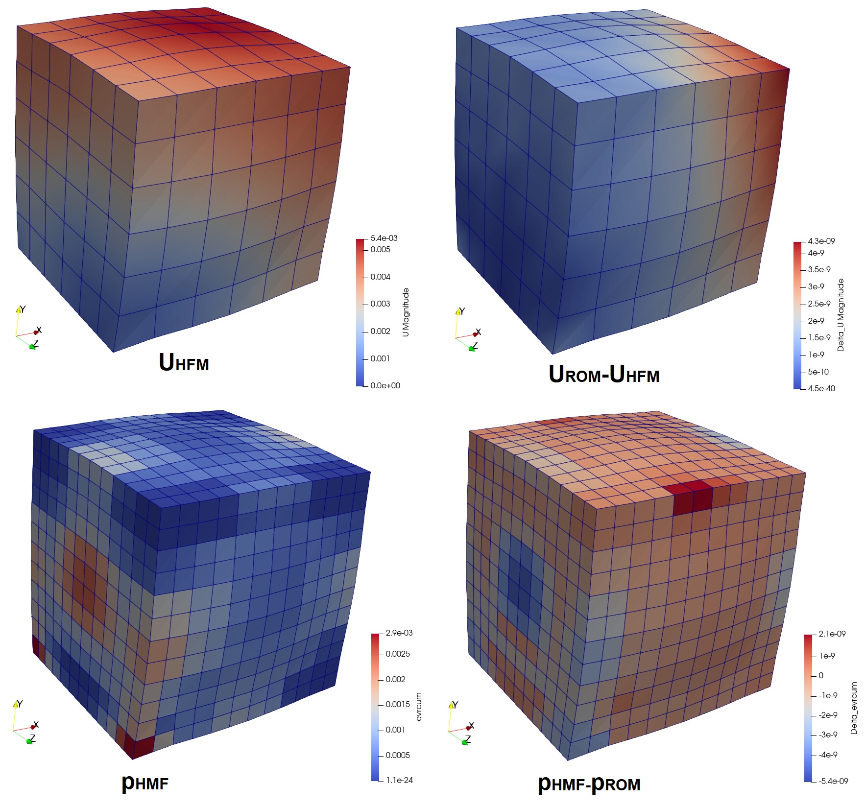
Fig. 5 Comparison between the reduced and reference high-fidelity solutions: (top) on the displacement U, (bottom) on the accumulated plasticity p.