MecaSequentialNoZsetLocalBasis

This use case aims to validate the methodology POD + ECM for uniform isotropic elactic material computations with Z-set, see Section Publications, article 1. In this linear case, the ECM should find a trivial quadrature formula, since the operators can be completely precomputed in the offline stage. This tutorial illustrates in particular how to include data from more than one HFM computation, and how to construct local reduced-order bases (ROB).

No optional prerequisite.

The data needed to execute the tutorials below can be loaded here: exampleMecaSequentialNoZsetLocalBasis.zip

Features: construct 2 local-ROBs from 2 HFM simulations with linear materials

The physical setting is the same as in the tutorial MecaSequential, except that there is no thermal loading in this case.

Moreover, the workflow illutrate the capacity of the library to deal with data from various HFM, and to deal with multiple local ROB.

Offline stage

First, we define a list that will contain two objects collectionProblemData, one for each of the two local ROB to be constructed:

collectionProblemDatas = []

for i in range(2):

The rest if the commented code for the offline stage is in this loop on i.

For each local ROB, we start by initiating a collectionProblemData:

collectionProblemData = CPD.CollectionProblemData()

collectionProblemData.AddVariabilityAxis('config',
                                        str,
                                        description="dummy variability")
collectionProblemData.DefineQuantity("U", "displacement", "m")
collectionProblemData.DefineQuantity("sigma", "stress", "Pa")


collectionProblemDatas.append(collectionProblemData)

Then, set up two problemData which we populate with data from two HFM computations, either from the early time steps (i=0 for the first local ROB), or from the late time steps (i=1 for the second local ROB).

folders = [folder0+"Computation1"+os.sep, folder0+"Computation2"+os.sep]

for j, folder in enumerate(folders):

    solutionReader = ZSR.ZsetSolutionReader(folder+solutionFileName)

    solutionU = S.Solution("U", nbeOfComponentsPrimal, numberOfNodes, primality = True)
    solutionSigma = S.Solution("sigma", nbeOfComponentsDual, numberOfIntegrationPoints, primality = False)
    outputTimeSequence = solutionReader.ReadTimeSequenceFromSolutionFile()
    if i==0:
        outputTimeSequence = outputTimeSequence[:len(outputTimeSequence)//2+2]
    elif i==1:
        outputTimeSequence = outputTimeSequence[len(outputTimeSequence)//2-2:]

    problemData = PD.ProblemData("case-"+str(i)+"_"+str(j))
    problemData.AddSolution(solutionU)
    problemData.AddSolution(solutionSigma)

    collectionProblemData.AddProblemData(problemData, config="case-"+str(i)+"_"+str(j))

    for time in outputTimeSequence:
        U = solutionReader.ReadSnapshot("U", time, nbeOfComponentsPrimal, primality=True)
        solutionU.AddSnapshot(U, time)
        sigma = solutionReader.ReadSnapshot("sig", time, nbeOfComponentsDual, primality=False)
        solutionSigma.AddSnapshot(sigma, time)

Then, set up two problemData which we populate with data from two HFM computations, either from the early time steps (i=0 for the first local ROB), or from the late time steps (i=1 for the second local ROB).

SP.CompressData(collectionProblemData, "U", 1.e-4, snapshotCorrelationOperator["U"] )

Mechanical.CompressOperator(collectionProblemData, operatorPreCompressionData, mesh, 1.e-3)

print("check compression...")
reducedOrderBasis = collectionProblemData.GetReducedOrderBasis("U")
collectionProblemData.CompressSolutions("U", snapshotCorrelationOperator["U"])

Compression errors are computed and printed. These lines illustrate how to declare a new Solution object, populate it with reduced coordinates, and uncompress them to express the reduced solution in the high-dimensional space.

compressionErrors = []
for j, folder in enumerate(folders):
    problemData = collectionProblemData.GetProblemData(config="case-"+str(i)+"_"+str(j))
    solutionU = problemData.GetSolution("U")
    outputTimeSequence = solutionU.GetTimeSequenceFromSnapshots()
    reducedCoordinatesU = solutionU.GetReducedCoordinates()
    solutionUApprox = S.Solution("U", nbeOfComponentsPrimal, numberOfNodes, primality = True)
    solutionUApprox.SetReducedCoordinates(reducedCoordinatesU)
    solutionUApprox.UncompressSnapshots(reducedOrderBasis)
    for t in outputTimeSequence:
        approxSolution = solutionUApprox.GetSnapshotAtTime(t)
        exactSolution = solutionU.GetSnapshotAtTime(t)
        norml2ExactSolution = np.linalg.norm(exactSolution)
        if norml2ExactSolution != 0:
            relError = np.linalg.norm(approxSolution-exactSolution)/norml2ExactSolution
        else:
            relError = np.linalg.norm(approxSolution-exactSolution)
        compressionErrors.append(relError)
print("compressionErrors =", compressionErrors)

Finally, change-of-basis matrices for converting reduced coordinates from one local ROB to the other are computed, and data is stored on disk for re-use in the online stage.

for i in range(2):

    dataCompressionData = {}
    for j in [j for j in range(2) if j != i]:
        reducedOrderBasisJ = collectionProblemDatas[j].GetReducedOrderBasis("U")
        dataCompressionData["projectedReducedOrderBasis_"+str(j)] = \
            collectionProblemDatas[i].ComputeReducedOrderBasisProjection("U", \
            reducedOrderBasisJ, snapshotCorrelationOperator["U"])

    collectionProblemDatas[i].AddDataCompressionData("U", dataCompressionData)

    SIO.SaveState("mordicusState_Basis_"+str(i), collectionProblemDatas[i])

Online stage

We illustrate below how the online problem is solved, with a switch between two local ROBs, all in complexity independent of the high-fidelity dimension.

onlineReducedCoordinates = []

for i in range(2):

    for loading in onlineProblemData.GetLoadingsForSolution("U"):
        loading.ReduceLoading(mesh, onlineProblemData, reducedOrderBases[i], operatorCompressionDatas[i])

    onlineCompressedSolution = Mechanical.ComputeOnline(onlineProblemData, timeSequences[i], operatorCompressionDatas[i], 1.e-4)

    onlineReducedCoordinates.append(onlineCompressedSolution)

    for t, reducedCoordinates in onlineReducedCoordinates[i].items():
        onlinesolution.AddReducedCoordinates(reducedCoordinates, t)

    if i==0:
        previousTime = timeSequences[i][-1]

        projectedReducedOrderBasis = collectionProblemDatas[0].GetDataCompressionData("U")["projectedReducedOrderBasis_1"]
        onlinesolution.ConvertReducedCoordinatesReducedOrderBasisAtTime(projectedReducedOrderBasis, previousTime)
        onlineProblemData.GetInitialCondition().SetReducedInitialSnapshot("U", onlinesolution.GetReducedCoordinatesAtTime(previousTime))

In the last 3 lines, the reduced coordinated of the online solution are converted from the first ROB to the second, and these converted reduced coordinates are set as an initial condition for the second local ROB online resolution.

Results

The ECM selects 2 reduced integration points in each of the 2 constructed local ROB. (this can slightly vary due the probabilistic nature of our implementation for ECM)

In Fig. 15, the quality of the reduced model is illustrated by comparing it to the high-fidelity reference. The comparison is done on the displacement, since no internal variable is available with the simple considered material.

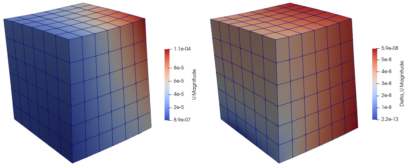
Fig. 15 Illustration of the ROM accuracy on the displacement U (left) HFM, (right) pointwise difference between the ROM and the HFM.